Multispectral vs Hyperspectral Satellite Imagery Explained
Multispectral vs hyperspectral satellite imagery: what changes when a sensor captures 200 bands instead of 4? Resolution trade-offs, costs, and which to choose.
Summary
- The multispectral vs hyperspectral question comes down to breadth versus depth. Multispectral captures 4-16 broad bands and remains the workhorse of commercial Earth observation, powering vegetation indices, land-use classification, and change detection at resolutions down to 0.3 metres.
- Hyperspectral sensors capture 20-200+ narrow, contiguous bands, enabling identification of specific materials, minerals, and vegetation species that multispectral can’t distinguish.
- The core trade-off is spatial resolution vs spectral detail. Commercial multispectral delivers 0.3-3m pixels. Most hyperspectral satellites sit at 5-30m.
- Commercial hyperspectral satellite data became widely available in 2024-2025, with Wyvern’s Dragonette constellation (5.3m, 23-32 bands) joining research missions like PRISMA, EnMAP, and NASA’s EMIT.
- Most projects need multispectral. Hyperspectral becomes worth the investment when you need to identify what something is, not just where it is.
Here’s something odd about the colour green.
To your eyes, a healthy wheat field and a paddock full of invasive weeds look almost identical. Same shade. Same vibe. A standard multispectral satellite can confirm they’re both vegetation, picking up chlorophyll absorption in the red and near-infrared bands without breaking a sweat. But it can’t tell you which is the crop and which is the weed.
A hyperspectral sensor can.
That distinction is worth serious money to the right buyer. Wheat from weeds, hematite from goethite, healthy coral from bleached coral. It all comes down to one thing: how many slices of the electromagnetic spectrum your sensor captures. The multispectral vs hyperspectral question gets asked constantly, and the honest answer is “you probably need multispectral.” But “probably” isn’t good enough when you’re spending thousands on satellite data, so let’s actually break down what these terms mean, where the trade-offs bite, and when hyperspectral genuinely justifies the extra cost.
The Imaging Spectrum: Panchromatic to Hyperspectral
Before we compare multispectral and hyperspectral, it helps to see where they sit on the broader spectrum of optical satellite imaging.
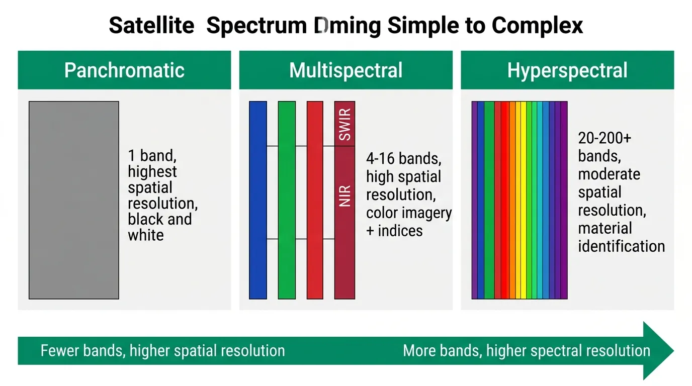
Panchromatic sensors capture a single, wide band spanning most of the visible spectrum. One band. Maximum spatial resolution. Black and white. WorldView-3 achieves 0.31m resolution in panchromatic mode. You can count cars in a parking lot, but you can’t tell a red one from a blue one.
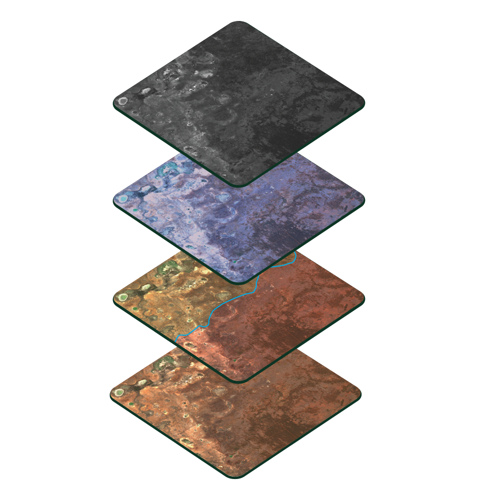
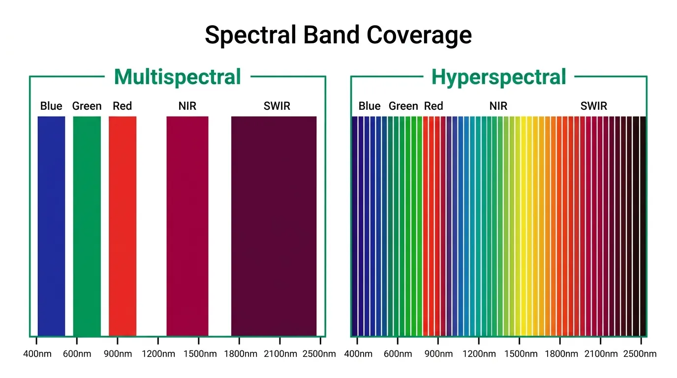
Multispectral sensors split the spectrum into 4-16 discrete bands, typically blue, green, red, near-infrared (NIR), and sometimes short-wave infrared (SWIR). Each band is 40-200nm wide. This is what most commercial satellites do. Sentinel-2 captures 13 bands at 10-60m resolution. WorldView-3 captures 16 bands (including 8 SWIR) at 1.24m multispectral resolution. Planet’s SuperDove fleet captures 8 bands at 3m. These sensors sample the spectrum at specific, strategically chosen wavelengths.
Hyperspectral sensors take a fundamentally different approach. Instead of sampling a few broad chunks of the spectrum, they capture dozens to hundreds of narrow, contiguous bands, each just 5-20nm wide. No gaps between them. Think of it as the difference between sampling a song at five points versus recording the entire track from start to finish.
How Multispectral Imaging Actually Works
A multispectral sensor is selective by design. It captures specific wavelength ranges that scientists have determined are useful for particular types of analysis. The near-infrared band is included because healthy vegetation reflects NIR strongly. That’s where NDVI and other vegetation indices come from.
The gaps between bands aren’t a limitation. They’re a deliberate engineering choice. By capturing fewer, wider bands, multispectral sensors collect more light per band, which means higher spatial resolution and a better signal-to-noise ratio. For most applications, that’s the right trade-off.
What multispectral does well:
- Vegetation health monitoring using NDVI, EVI, and SAVI indices calculated from red and NIR bands. This is the backbone of precision agriculture and forestry monitoring globally.
- Land cover classification to distinguish water, urban areas, vegetation, and bare soil. Four or five bands is plenty.
- Change detection by comparing imagery from different dates to spot construction, deforestation, flooding, or urban expansion.
- Water quality assessment using blue and green bands to reveal turbidity, algal blooms, and sediment concentration.
What multispectral can’t do: tell you which species of vegetation is stressed, or which specific mineral is in that exposed rock face, or which chemical contaminated that waterway. All green vegetation looks roughly the same in 4-8 bands. You know it’s there. You just don’t know what it is.
How Hyperspectral Imaging Works
Hyperspectral sensors capture the full spectral curve of every pixel. Where a multispectral sensor gives you five or ten data points along the electromagnetic spectrum, a hyperspectral sensor gives you two hundred.
Why does that matter?
Because every material on Earth has a unique spectral signature. A specific pattern of how it absorbs and reflects different wavelengths based on its molecular composition. Chlorophyll absorbs red light and reflects NIR. Iron oxide absorbs around 900nm. Calcite has a distinctive absorption feature near 2,300nm.
With enough spectral detail, you can identify these absorption features and match them against known spectral libraries. That’s how a geologist can distinguish hematite (Fe₂O₃) from goethite (FeOOH) from 600 kilometres above the Earth. They look the same colour to the naked eye but have completely different spectral curves between 800-1000nm.
What hyperspectral does that multispectral can’t:
- Mineral identification to distinguish individual mineral species in exposed rock and soil. Copper carbonate, gypsum, kaolinite, alunite — each has unique absorption features only visible in narrow bands.
- Vegetation species discrimination that can tell eucalyptus from acacia from pine. Not just “it’s green” but “it’s this specific green.”
- Soil composition mapping to identify organic carbon content, moisture levels, clay mineralogy, and contamination.
- Water constituent analysis that detects specific phytoplankton species, dissolved organic matter, and individual pollutant types.
- Gas emission detection for methane, CO₂, and other greenhouse gases with spectral absorption signatures that hyperspectral sensors can pick up.
Multispectral vs Hyperspectral: The Key Differences
Here’s where the comparison gets concrete.
| Feature | Multispectral | Hyperspectral |
|---|---|---|
| Spectral bands | 4-16 bands | 20-200+ bands |
| Band width | 40-200nm (broad) | 5-20nm (narrow) |
| Band arrangement | Discrete, with gaps | Contiguous, no gaps |
| Best commercial spatial resolution | 0.31m pan / 1.24m MS (WorldView-3) | 5.3m (Wyvern Dragonette) |
| Typical spatial resolution | 0.5-10m | 5-30m |
| Data volume per scene | Moderate (4-16 layers) | Very large (100-200+ layers) |
| Processing complexity | Standard GIS tools | Specialist spectral analysis software |
| Primary strength | Where things are | What things are |
| Approximate cost | $2-55/km² (archive) | $10-80/km² (varies by provider) |
| Commercial availability | Abundant (dozens of constellations) | Limited but growing fast |
The spatial resolution gap is the thing that trips people up. If you need to count individual trees, multispectral at 0.5m beats hyperspectral at 30m every time. But if you need to know which trees are Eucalyptus camaldulensis and which are Eucalyptus globulus, the spectral detail wins, even at lower spatial resolution.
Data volume is the other big consideration. A single hyperspectral scene might be 10-50x larger than the equivalent multispectral image. More storage, more processing time, more specialised software. Standard GIS packages handle multispectral data out of the box. Hyperspectral analysis typically requires tools like ENVI, or custom Python workflows using libraries like spectral or hyperspy.
When to Use Which: A Decision Framework
Don’t default to hyperspectral because it sounds fancier. It isn’t always better. It’s different.
Use multispectral when you need:
- High spatial resolution (sub-metre)
- Frequent revisit for time-series monitoring
- Standard index calculations (NDVI, NDWI, NDMI)
- Land cover classification and change detection
- Cost-effective coverage of large areas
- Quick turnaround and simple processing
Use hyperspectral when you need to:
- Identify specific minerals in mining exploration or environmental assessment
- Discriminate between similar plant species for biodiversity mapping or invasive species detection
- Map soil properties like organic carbon, clay content, or contamination levels
- Detect subtle crop stress before it shows up in standard NDVI
- Monitor specific water pollutants or algal species
- Quantify atmospheric gas concentrations
Consider using the two together when the project demands it. A mining company might use multispectral imagery at 0.5m to map the site layout and track physical changes monthly, then task a hyperspectral collection once or twice a year to assess mineral composition in tailings and monitor vegetation species during rehabilitation. That layered approach gets you spatial precision and spectral depth without blowing the budget on either.
Commercial Hyperspectral Satellites in 2026
For a long time, hyperspectral satellite data meant waiting months for access to research missions with restrictive licences and 30m resolution at best. That picture has changed.
Currently operational:
- Wyvern Dragonette (Dragonette-001 to -004): 5.3m GSD, 23-32 bands in the VNIR range (400-1000nm). The highest-resolution commercial hyperspectral constellation flying today. Wyvern, a Canadian company founded in 2018, has Dragonette-005 and -006 scheduled for launch later in 2026. Geopera is a Wyvern distribution partner, offering Dragonette data through our imagery platform.
- PRISMA (ASI, Italy): 30m resolution, 239 bands covering 400-2505nm across VNIR and SWIR. Operational since 2019. Free for research use through the Italian Space Agency.
- EnMAP (DLR, Germany): 30m resolution, 242 bands covering 420-2450nm. Launched April 2022. Data available through DLR’s EOWEB GeoPortal.
- EMIT (NASA/JPL): 60m resolution, 285 bands covering 380-2500nm. Mounted on the International Space Station since July 2022. Originally designed for mineral dust source mapping, but all data is publicly accessible through NASA Earthdata.
- DESIS (DLR/Teledyne): 30m resolution, 235 bands covering 400-1000nm (VNIR only). Also mounted on the ISS.
Compared to multispectral availability, hyperspectral options are still limited. Dozens of multispectral constellations orbit Earth right now. Sentinel-2, Landsat 9, WorldView-3, Beijing-3, Jilin-1, Planet SuperDove. They cover the planet daily at resolutions from 0.3m to 10m. Hyperspectral doesn’t have that density yet. Wyvern’s constellation expansion and new commercial entrants will change the equation over the next two to four years, but today, getting cloud-free hyperspectral data over a specific area still requires more planning and patience than pulling multispectral from an archive.
Hyperspectral vs Multispectral Processing: What You’re Signing Up For
Something the typical comparison article never tells you: the processing burden is wildly different between hyperspectral and multispectral data.
Multispectral processing is well-understood territory. Orthorectification, atmospheric correction, pansharpening, index calculation. These are standard workflows that any competent imagery provider handles as part of delivery. When you order satellite imagery that’s multispectral, you can reasonably expect analysis-ready data that loads straight into QGIS or ArcGIS.
Hyperspectral processing is a different animal. Beyond the standard geometric and atmospheric corrections, you’ll typically need:
- Noise reduction across hundreds of bands (atmospheric water vapour absorption creates noisy bands that need masking or interpolation)
- Dimensionality reduction using Principal Component Analysis (PCA) or Minimum Noise Fraction (MNF) transforms to identify the most information-rich band combinations
- Spectral unmixing, because most hyperspectral pixels at 30m contain a mix of materials. Unmixing algorithms decompose each pixel into its constituent materials and their proportions.
- Spectral library matching to compare pixel signatures against reference databases (like the USGS Spectral Library) and identify materials
This isn’t a few clicks in QGIS. It’s specialist work that requires someone comfortable with ENVI, Python spectral analysis libraries, or similar tools. Without that expertise, the data just sits on a hard drive doing nothing.
The practical takeaway: factor processing capability into your decision. The cost of satellite imagery isn’t just the acquisition price. It’s acquisition plus the expertise to turn 200 bands of raw data into actionable information. If you don’t have that in-house, find a provider who handles it.
How We Handle This at Geopera
We work across the full optical spectrum. Our platform connects you to multispectral sensors from Vantor (formerly Maxar), 21AT’s Beijing-3, CGSTL’s Jilin-1, SpaceWill’s SuperView, and Sentinel-2, plus Wyvern’s Dragonette constellation for hyperspectral. We also maintain over 350 spectral indices on our documentation site, calculated and documented with code samples.
Every order goes through our processing pipeline: orthorectification, atmospheric correction, pansharpening where applicable. That processing is included, not an add-on. Whether you need a 0.3m multispectral scene for infrastructure monitoring or a 5.3m hyperspectral capture for mineral exploration, you get analysis-ready data.
Not sure which type fits your project? See how we deliver both multispectral and hyperspectral data, processed and analysis-ready, through our satellite imagery platform.
Frequently Asked Questions
What is the difference between multispectral and hyperspectral satellite imagery?
Multispectral sensors capture 4-16 broad, non-contiguous spectral bands (40-200nm wide each), optimised for general-purpose Earth observation like vegetation monitoring and land classification. Hyperspectral sensors capture 20-200+ narrow, contiguous bands (5-20nm wide each), enabling identification of specific materials through their unique spectral absorption signatures. In practical terms, multispectral tells you where things are; hyperspectral tells you what they are.
How does hyperspectral imaging work?
Hyperspectral sensors record reflected sunlight across hundreds of narrow, adjacent wavelength bands, producing a complete spectral curve for every pixel. Each material on Earth absorbs and reflects light differently at specific wavelengths due to its molecular composition. Analysts compare these per-pixel spectral curves against known reference libraries to identify the chemical composition and physical properties of surface materials from orbit.
Is hyperspectral satellite imagery commercially available in 2026?
Yes. Commercial hyperspectral data is available from Wyvern’s Dragonette constellation at 5.3m resolution with 23-32 VNIR bands, accessible through providers including Geopera. Free research-grade data is available from PRISMA (30m, 239 bands), EnMAP (30m, 242 bands), and NASA’s EMIT (60m, 285 bands). Commercial availability remains more limited than multispectral but is expanding as Wyvern and others grow their constellations.
When should I choose hyperspectral over multispectral?
Choose hyperspectral when your analysis requires material identification rather than spatial mapping. That means mineral exploration, vegetation species discrimination, soil composition analysis, water quality constituent detection, or atmospheric gas monitoring. For change detection, land cover classification, general vegetation health monitoring, or any application requiring sub-metre resolution, multispectral is the better and more cost-effective choice.
What spatial resolution do hyperspectral satellites achieve?
The highest-resolution commercial hyperspectral satellite in 2026 is Wyvern’s Dragonette at 5.3m ground sampling distance (GSD). Research missions like PRISMA and EnMAP operate at 30m, and NASA’s EMIT at 60m. For comparison, leading multispectral satellites achieve 0.31m (WorldView-3 panchromatic) to 3m (Planet SuperDove). The resolution gap exists because capturing more spectral bands means each detector element collects less light per band, reducing signal strength at finer spatial scales.
Related Articles
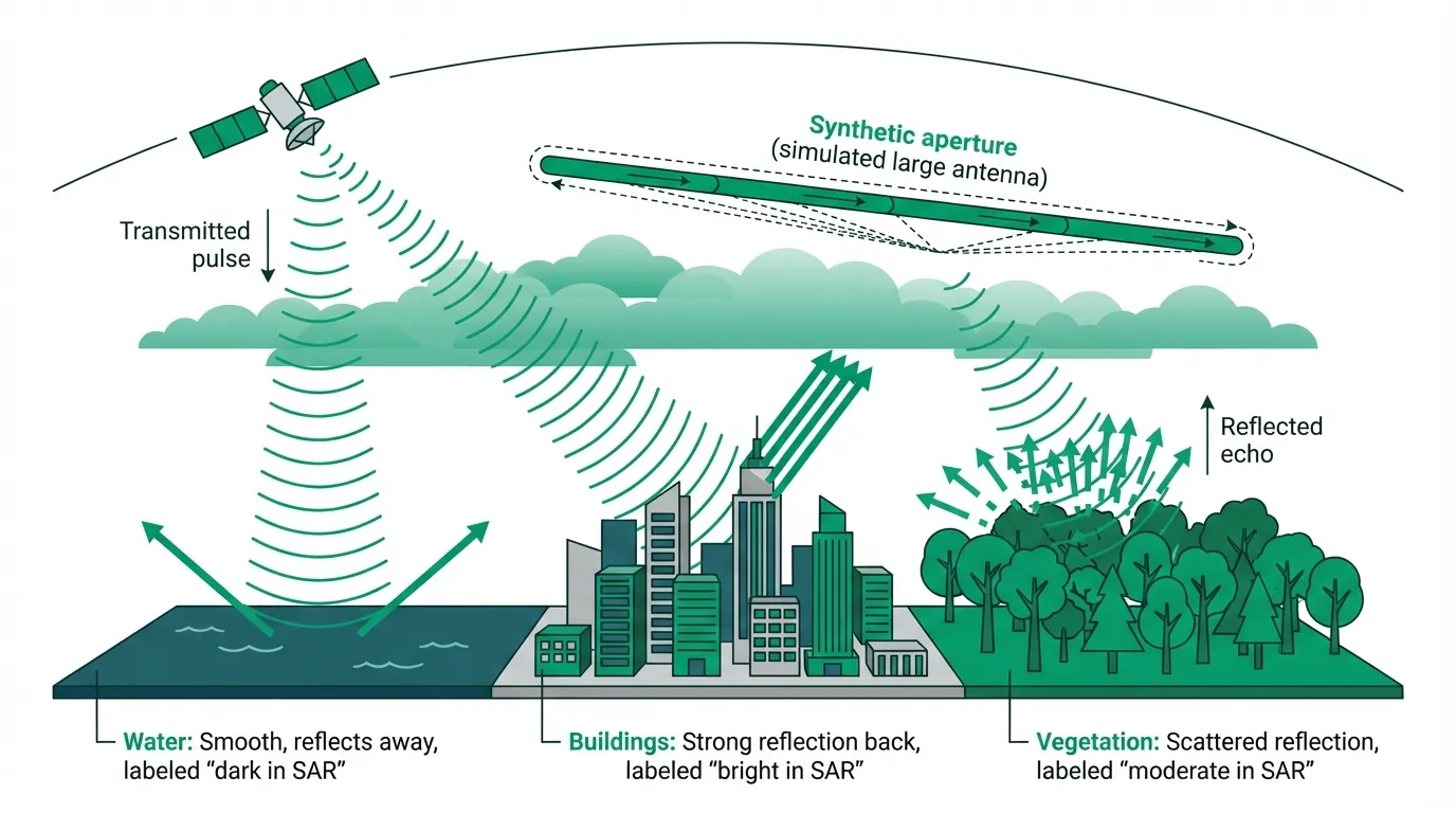
What is SAR Satellite Imagery? How Radar Sees What Optical Can't
SAR satellites use radar to image Earth through clouds, at night, in any weather. How synthetic aperture radar works and which satellites to use.

What You Should Know About Optical Satellite Imagery
How optical satellite imagery works, from spectral bands to spatial resolution, plus practical applications across industries.